The Nim Ray Tracer Project — Part 4: Calculating box normals

I needed a way to calculate normals for the box primitive in my ray tracer. Of course, this is trivial if the boxes are represented as a triangle meshes with stored per vertex normals—just use the triangle intersection routine and job done! Interestingly, all online resources I could find either suggest this approach or some naive algorithm that intersects the ray with all the six planes that define the box… Ughh, we can certainly do better than that!

First of all, because we’re not dealing with arbitrary boxes in 3D space here, we can make certain optimisations. For my case, I wanted to be able to calculate the normals for axis-aligned bounded boxes (AABBs) only that are defined just by their two diagonally opposite points.

Why just AABBs? What about boxes that are not parallel to the axes? Well, the way I’m doing things is that the final world position of an object is described by its objectToWorld transform matrix that can include rotation as well. Using AABBs for boxes, unit spheres for spheres etc. simplifies the intersection routines a lot (makes them faster to calculate). Then during rendering, I’m using the inverse transform worldToObject to transform the ray to object space and do the intersection there¹. This method is vastly more efficient for triangle meshes as well—we only need to inverse transform a single ray instead of transforming potentially thousands or millions of triangles!

This is how our geometry definitions look like in Nim (we’re using nim-glm for the vector maths stuff). We’re going to use AABBs later for constructing bounding volume hierarchies (BVH) as well, hence the separate AABB and Box types.

import glm

type
  AABB* = ref object
    vmin*, vmax*: Vec4[float]

type
  Geometry* = ref object of RootObj
    objectToWorld*: Mat4x4[float]
    worldToObject*: Mat4x4[float]

  Sphere* = ref object of Geometry
    r*: float

  Plane* = ref object of Geometry
    discard

  Box* = ref object of Geometry
    aabb*: AABB

Box normal algorithm

We’ll solve the problem for the unit cube first, then we’ll find a way to map the solution from an arbitrary AABB to the unit cube. For the sake of simplicity, we’re going to illustrate the basic algorithm in 2D only; extending it to 3D is trivial.

Solution for the unit cube

Consider the blue $P$ points that lie on the rectangle in Figure 1. By looking at the vectors pointing to these points (blue arrows), we can make the observation that by taking the integer parts of the vectors' coordinates (not rounding!), we would get the normals we’re after (green arrows). And that’s it!

There are some complications though. This approach yields perfectly correct results for $P_1$, $P_2$ and $P_3$, but for $P_4$ we’d get $(1, -1)$, which firstly is not a normal, and secondly, is diagonal. Strictly speaking, the diagonal-ness is a bit incorrect, although it can be argued that the normals are “undefined” at the corners, thus the diagonal could as well be accepted as a valid answer. Either way, in practice this won’t make any difference—we will very rarely hit the corners exactly, and even if we did, the “degenerate” normals will be averaged out with the “normal” ones during multi-sampling. We just need to normalise our resulting vector after the integer truncation to ensure that the length is always 1.

Of course, we can always put a few if statements at the end to filter out the diagonals, but that would make the whole algorithm slower. It’s also worth mentioning that in 3D we will have edge cases too in addition to the corner cases (no pun intended).

Solution for arbitrary AABBs

Mapping the problem from an AABB to the unit cube is basically a translation and scaling exercise. Our AABB is defined by its two diagonally opposite points, $V_{\min}$ and $V_{\max}$, from which we can easily calculate its centre point $C$ (now in 3D):

$$ C=⟨{V_{\min_\x} + V_{\max_\x}} / 2, {V_{\min_\y} + V_{\max_\y}} / 2, {V_{\min_\z} + V_{\max_\z}} / 2⟩$$

Next, we’ll calculate the vector $p↖{→}$ that points from the centre point to the hit point $P_{\hit}$:

$$ p↖{→} = P_{\hit} - C $$

This vector corresponds to the blue vectors in Figure 1. What we need to do next is map $p↖{→}$ to the unit cube by calculating divisor values for each of its dimensions:

$$ \d_x = {\abs(V_{\min_\x}-V_{\max_\x})} / 2 $$ $$ \d_y = {\abs(V_{\min_\y}-V_{\max_\y})} / 2 $$ $$ \d_z = {\abs(V_{\min_\z}-V_{\max_\z})} / 2 $$

From $p↖{→}$ and the scalar divisors $\d_x$, $\d_y$ and $\d_z$ we can calculate the normal $n↖{→}$ at the hit point (the green vectors in Figure 1):

$$ n↖{→} = ⟨\int(p_\x / \d_x), \int(p_\y / \d_y), \int(p_\z / \d_z)⟩ $$

Implementation

Okay, time to have a look at some Nim code! This is a slightly optimised version of the above algorithm:

method normal*(b: Box, hit: Vec4[float]): Vec4[float] =
  let
    c = (b.aabb.vmin + b.aabb.vmax) * 0.5
    p = hit - c
    d = (b.aabb.vmin - b.aabb.vmax) * 0.5
    bias = 1.000001

  result = vec(((p.x / abs(d.x) * bias).int).float,
               ((p.y / abs(d.y) * bias).int).float,
               ((p.z / abs(d.z) * bias).int).float).normalize

Wait a minute, what’s that multiplier bias doing there? That, my friend, is the amount of difference between theory of practice. For educational purposes only, this is what we would get if we left it off:

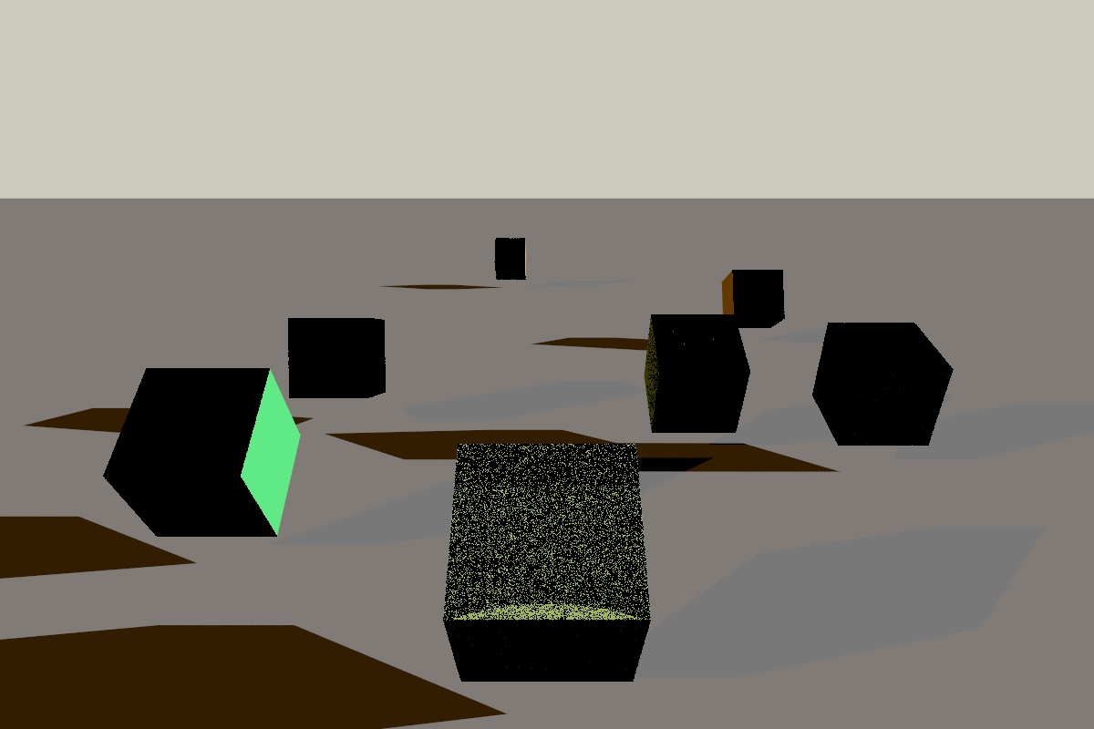
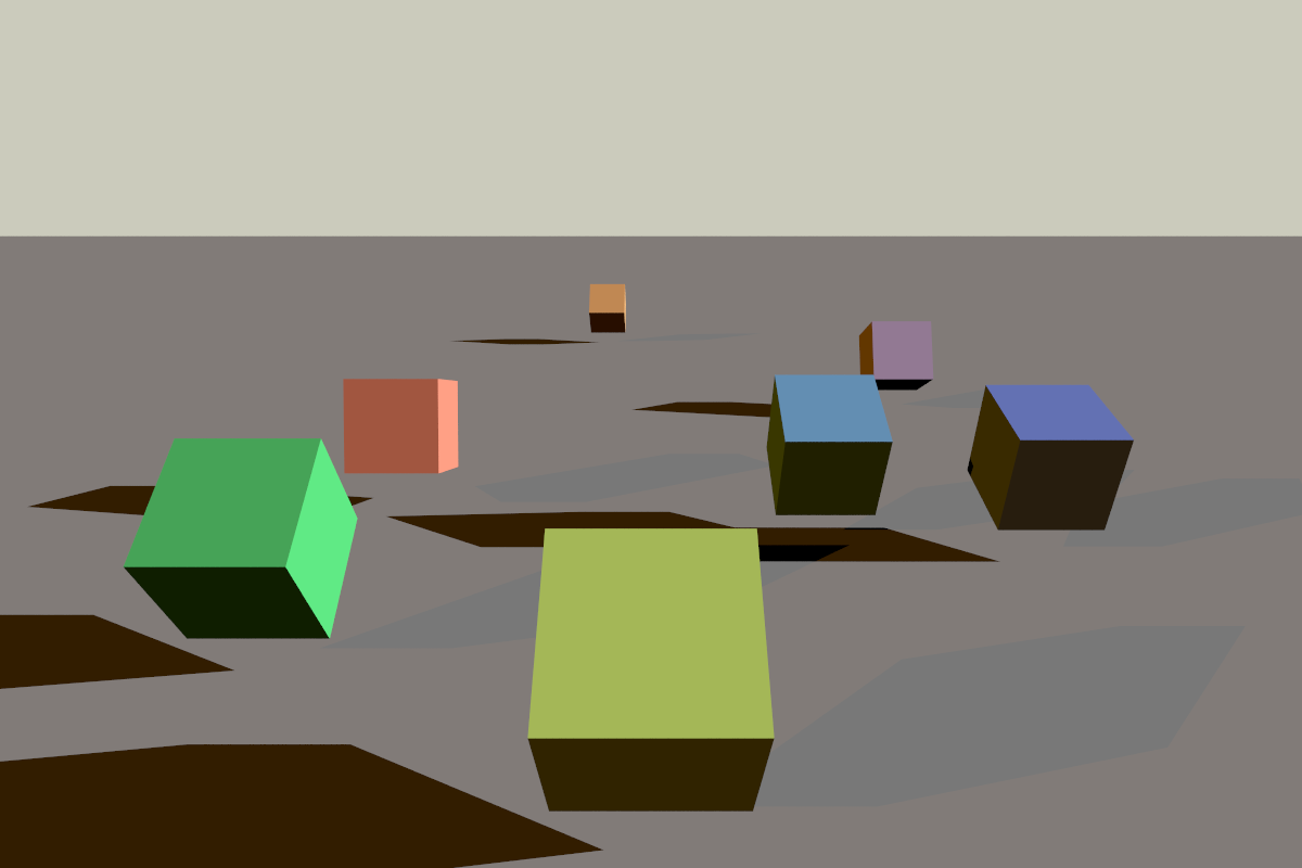
Ooops, not exactly the result we were hoping for! What’s going on here? The problem is that because of floating point inaccuracies, our final coordinates that are supposed to be 1.0 will sometimes end up being a bit less than that, say 0.999999994, and in the final casting to int step they will become 0 instead of 1. To fix this, we’ll need to nudge the points a tiny bit outwards by scaling them up by a multiplicative epsilon value. The good news is that this bias value doesn’t have to be terribly accurate; we’re going to truncate the decimals away anyway. With this fix in place, we’ll get the correct results:

Correctness vs real life

As I explained above, although this fast normal calculation method can be considered incorrect by the mathematician types (and perhaps it is, I don’t know for sure), it seems to work perfectly fine for practical purposes. At least, I couldn’t spot any unwanted artefacts on my test renders, and theoretically, there’s very little chance to run into those diagonal normals, and even then, their contribution to the final image would be minimal.

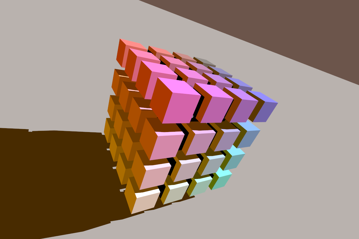
In parting, here is a more complex scene to prove my point. If anyone is aware of a situation where this algorithm could cause problems, I am interested to hear about it though!