The Nim Ray Tracer Project — Part 3: Lighting & Vector Maths

Ok, so last time I ended my post with the cliffhanger that I’m going to show some actual Nim code in the next episode, which is this. Well, I’ll never make foolish promises like that again, I swear! Now I need to come up with some good excuses why we’re gonna do something slightly different instead…

But seriously, I don’t think there’s much point in dissecting my code line by line here, it would be just a colossal waste of time for everyone involved and the codebase is in constant flux anyway. Anyone who’s interested can take a look at the code in the GitHub repository. What we’ll do instead from here on is discuss some of my more interesting observations about ray tracing on a higher level and maybe present the occasional original trick or idea I managed to come up with.

Idealised light sources

The teaser image at the end of the last post used a very simple shading mechanism called facing ratio shading for the spheres. As the name implies, that just relies on the angle between the ray direction and the surface normal at the ray hit location. This looks really basic, although it still might come in handy sometimes for debugging.

A more useful shading method is the so called diffuse or Lambertian shading that simulates how diffusely reflecting, or matte surfaces behave in real life. Realistic shaders require light sources though, so the next thing to implement is some sort of lighting. We’re doing ray tracing kindergarten here, so the first light types to implement will be idealised directional and point lights.

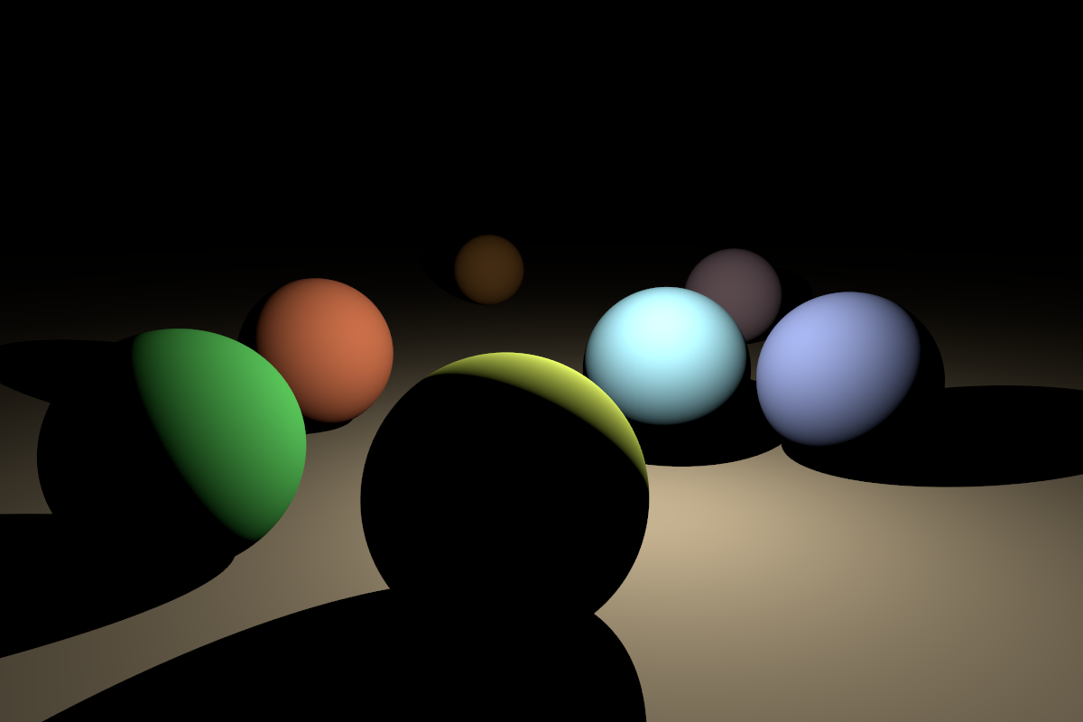
Directional lights (or distant lights) are light sources that are infinitely far away, hence they only have direction but no position, and most importantly, no falloff. Light sources of this kind are therefore ideal for simulating the sun or other celestial light emitting objects that are “very far away”. Shadows cast by directional lights are always parallel. This is how the example scene from the previous post looks like when illuminated by two directional lights:

Point lights are idealised versions of light sources that are relatively small in size and emit light in all directions, therefore they only have position but no direction. From this follows that point lights cast radial shadows. In contrast with directional lights, point lights do exhibit falloff (light attenuation), which follows the well-known inverse-square law. Good examples of point lights are light bulbs, LEDs or the candlelight. Of course, in real life these light sources do have an actual measurable area, but we’re not simulating that (yet). Note how drastically different the exact same scene looks like when illuminated by a single point light:

Again, all this shading stuff in explained in great detail in the shading lesson at Scratchapixel, so refer to that excellent article series if you’re interested in the technical details.

It is very important to note that lighting must always be calculated in linear space in a physically-based renderer. That’s how light behaves in the real world; to calculate the effects of multiple light sources on a given surface point, we just need to calculate their contribution one light at a time and then simply sum the results. What this means is that the data in our internal float framebuffer represents linear light intensities that we need to apply sRGB conversion to (a fancy way of doing gamma-encoding) if we want to write it to a typical 8-bit per channel bitmap image file. If you are unsure about what all this means, I highly recommend checking out my post on gamma that should hopefully clear things up.

Direct vs indirect illumination

What we’ve implemented so far is pretty much a basic classic ray tracer, or a path tracer, to be more exact, which works like this from a high-level perspective:

1. Primary rays are shot from the aperture of an idealised pinhole camera (a point) through the middle of the pixels on the image plane into the scene.

2. If a ray intersects with an object, we shoot a secondary shadow ray from the point of intersection (hit point) towards the light source (which are idealised too, as explained above).

3. If the path of the shadow ray is not obstructed by any other objects as it travels toward the light source, we calculate the light intensity reflected towards the view direction at the hit point with some shading algorithm, otherwise we just set it to black (because the point is in shadow). Due to the additive nature of light, handling multiple light sources is very straightforward; just repeat steps 2 & 3 for all lights and then sum the results.

The astute reader may have observed that there’s lots of simplification going on here. For a start, real world cameras and light sources are not just simple idealised points in 3D space, and objects are not just illuminated by the light sources alone (direct illumination), but also by light bounced off of other objects in the scene (indirect illumination). With our current model of reality, we can only render hard edged shadows and no indirect lighting. Additionally, partly because of the lack of indirect illumination in our renderer, these shadows would appear completely black. This can be more or less mitigated by some fill light tricks that harken back to the old days of ray tracing when global illumination methods weren’t computationally practical yet. For example, if there’s a green coloured wall to the left of an object, then put some lights on the wall that emit a faint green light to the right to approximate the indirect light rays reflected by the wall. This is far from perfect for many reasons; on the example image below I used two directional lights and a single point light as an attempt to produce a somewhat even lighting in the shadow areas, but, as it can be seen, this hasn’t completely eliminated the black shadows.

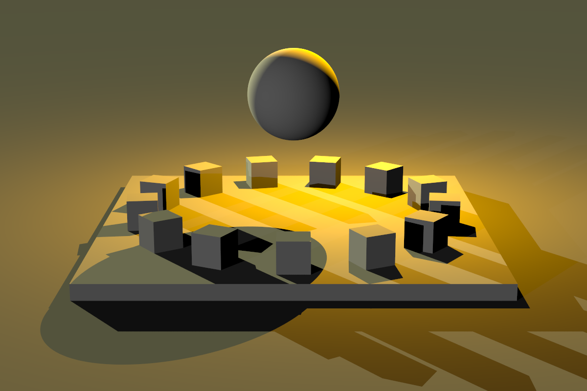
It’s easy to see how the number of lights can easily skyrocket using this approach, and in fact 3D artist have been known to use as many as 40-60 lights or more per scene to achieve realistic looking lighting without global illumination. As for the hard shadows, there’s no workaround for that at our disposal at the moment—soft shadows will have to wait until we are ready to tackle area lights.

Vector maths (addendum)

Before we finish for today, here’s some additional remarks regarding the vector maths stuff we discussed previously. I’m using the nim-glm library in my ray tracer, which is a port of GLM (OpenGL Mathematics), which is a maths library based on the GLSL standard. A quick look into the nim-glm sources reveals that the library uses row-major order storage internally:

var def = "type Vec$1*[T] = distinct array[$1, T]" % [$i]
var def = "type Mat$1 x$2*[T] = distinct array[$1, Vec$2[T]]" % [$col, $row]

We don’t actually need to know about this as long as we’re manipulating the underlying data structures through the library, but it’s good to be aware of it.

(If you’re confused now and think that row/column-major storage ordering has anything to do with coordinate system handedness or column versus row vector notation, this explanation should set you straight.)

Because we’re using column vector notation, which is the standard in mathematics, OpenGL and pbrt, we need to do a matrix-by-vector multiplication to transform a vector $v↖{→}$ by a matrix $\bo M$:

$$ v_t↖{→} = \bo M v↖{→} $$

vec3 v, u;
mat3 m;
u = v * m;

is equivalent to

u.x = dot(v, m[0]); // m[0] is the left column of m
u.y = dot(v, m[1]); // dot(a,b) is the inner (dot) product of a and b
u.z = dot(v, m[2]);

Also, the transforms have to be read “backwards”, e.g. the vector v below will be translated by 5 units along the z-axis first, then rotated by 60 degrees around the y-axis, and finally translated by -30 units along the x-axis:

let v: Vec4[float] = vec(1.0, 2.0, 3.0)

let m: Mat4x4[float] = mat4(1.0).translate(vec(-30.0, 0.0, 0.0))
                                .rotate(Y_AXIS, degToRad(60.0))
                                .translate(vec(0.0, 0.0, 5.0))

let vt = m * v

The function vec and the constant Y_AXIS are just some convenience stuff. We’re using homogeneous coordinates , so a Vec4[float] can denote both points and vectors. Points must have their 4th w component always set to 1.0 (otherwise translation would not work), and vectors to 0.0 (translation is undefined for vectors). The following definitions help with the construction of points and vectors and the conversion of one type into the other:

const X_AXIS* = vec3(1.0, 0.0, 0.0)
const Y_AXIS* = vec3(0.0, 1.0, 0.0)
const Z_AXIS* = vec3(0.0, 0.0, 1.0)

template vec*[T](x, y, z: T): Vec4[T] = vec4(x, y, z, 0.0)
template vec*[T](v: Vec4[T]): Vec4[T] = vec4(v.xyz, 0.0)

template point*[T](x, y, z: T): Vec4[T] = vec4(x, y, z, 1.0)
template point*[T](v: Vec4[T]): Vec4[T] = vec4(v.xyz, 1.0)

Storing the w component is convenient because we don’t need to constantly add it to the vector when transforming it by a 4x4 matrix. Some people would introduce distinct point and vector types, but I don’t think that’s worth the trouble; it would just complicate the code too much for dubious benefits.

Finally, the following checks can be useful when debugging with asserts (these could probably be improved by using an epsilon for the equality checks):

template isVec*[T]  (v: Vec4[T]): bool = v.w == 0.0
template isPoint*[T](v: Vec4[T]): bool = v.w == 1.0

Well, looks like in the end we did inspect some Nim code, after all! :)